Checking Monte Carlo convergence

Checking Monte Carlo convergence#

In Variational Monte Carlo the expectation values we compute are stochastic estimates that rely on the Markov chains being well-mixed and thermalized. When this is not the case, every quantity you compute — energies, gradients, observables — is unreliable, and your optimization may be solving the wrong problem.

However, it is customary in NQS training on GPUs to work with very short chains on which it is challenging to reliably estimate whether they are well mixed during training. In practice, if you tune it well this gives great speedups and does not hamper convergence, but you are travelling blindly and can’t know easily if MC is an issue or not.

NetKet provides two methods on MCState that help you diagnose and control sampling quality, which we will discuss in this page.

Method	Purpose
`check_mc_convergence()`	Diagnose chain mixing quality for a given operator
`thermalise()`	Advance chains to stationarity before measuring
`expect_to_precision()`	Sample until a target statistical error is reached

This guide explains when and how to use these tools.

Warning

All three methods are experimental and subject to change without notice in future NetKet releases. If you find them useful (or not!), please let us know with a 👍 / 👎 on GitHub or on Slack.

The chain-length problem in VMC#

At every VMC iteration, the sampler runs several Markov chains of length chain_length to generate samples used to estimate the energy and its gradient. Reliable sampling diagnostics — the Gelman-Rubin \(\hat{R}\) statistic and the integrated autocorrelation time \(\tau_\text{corr}\) — require chains of at least ~100 steps to be meaningful.

However, in practice, the chain length per iteration is often very short — typically 2 to 8 steps per chain — because:

Modern GPUs are efficient at running thousands of parallel chains simultaneously, so you amortise the fixed overhead over many chains rather than making each chain longer.
Each parameter update changes the wavefunction, so there is little benefit in running very long chains before updating.
During the optimization the wavefunction changes little step-to-step, so you effectively thermalise across small changes of parameters.

A typical setup might look like:

L = 20
g = nk.graph.Hypercube(length=L, n_dim=1, pbc=True)
hi = nk.hilbert.Spin(s=1 / 2, N=g.n_nodes)
ha = nk.operator.Ising(hilbert=hi, graph=g, h=1.0)
ma = nk.models.RBM(alpha=1, param_dtype=float)

# Many parallel chains (512), but each chain is only 2 steps long per iteration
# (1008 samples / 512 chains ≈ 2 steps/chain/iteration)
sa = nk.sampler.MetropolisLocal(hi, n_chains=512, sweep_size=L)
vs = nk.vqs.MCState(sa, ma, n_samples=1024, n_discard_per_chain=10)

print(f"Number of chains    : {vs.sampler.n_chains}")
print(f"Steps per chain     : {vs.chain_length}")
print(f"Total samples       : {vs.n_samples}")

Number of chains    : 512
Steps per chain     : 2
Total samples       : 1024

With chain_length = 2, the \(\hat{R}\) and \(\tau_\text{corr}\) estimates printed by vs.expect() at each step are unreliable — not enough data per chain to compute them. Despite this, the optimization can still converge, because the average over many short chains is still statistically valid (the bias is controlled by the parameter changes between steps, not by chain length).

Let us run a short VMC optimisation and look at what is logged:

import optax

op = optax.sgd(learning_rate=0.02)
gs = nk.driver.VMC_SR(
    ha,
    op,
    variational_state=vs,
    diag_shift=0.01,
)

log = nk.logging.RuntimeLog()
gs.run(n_iter=300, out=log)

Automatic SR implementation choice:  QGT
online_statistics: chain_length=2, decay=0.960

(RuntimeLog():
  keys = ['Energy', 'acceptance', 'Energy_ema'],)

The `Energy_ema` diagnostic during optimization#

When the chain length is short (less than ~50 steps), VMC_SR automatically accumulates local-energy samples across iterations using an exponential moving average (EMA) window. This effectively pools samples from multiple consecutive iterations to build a longer virtual chain, making \(\hat{R}\) and \(\tau_\text{corr}\) estimates meaningful even when each individual iteration has a very short chain.

The resulting running statistics are logged as Energy_ema alongside the usual Energy key:

Warning

The autocorrelation time so computed is not the standard autocorrelation time because the chain is not stationary! Similarly, the R_hat is also different from what Gellman had envisaged.

Those quantities are still meaningful most of the time, but they may break in some instances. Be a bit cautious, and if you think they are giving wrong hints, let us know.

iters = log.data["Energy"].iters
energy_mean = np.real(log.data["Energy"].Mean)
energy_err  = np.real(log.data["Energy"].Sigma)

fig, axes = plt.subplots(1, 3, figsize=(13, 4))

# Energy convergence
ax = axes[0]
ax.errorbar(iters, energy_mean, yerr=energy_err, fmt="-", lw=1, capsize=0, label="Energy")
ax.set_xlabel("Iteration")
ax.set_ylabel("Energy")
ax.set_title("Energy")
ax.legend(fontsize="small")

# R-hat from EMA
ax = axes[1]
rhat_ema = np.real(log.data["Energy_ema"].R_hat)
ax.plot(log.data["Energy_ema"].iters, rhat_ema, lw=1, color="C2", label=r"$\hat{R}$ (EMA)")
ax.axhline(1.05, color="gold",  lw=1.2, ls="--", label=r"$\hat{R}=1.05$ (warning)")
ax.axhline(1.10, color="salmon", lw=1.2, ls="--", label=r"$\hat{R}=1.10$ (bad)")
ax.set_xlabel("Iteration")
ax.set_ylabel(r"$\hat{R}$")
ax.set_title(r"Gelman-Rubin $\hat{R}$ (EMA)")
ax.legend(fontsize="small")

# tau from EMA (key in the log is "TauCorr")
ax = axes[2]
tau_ema = np.real(log.data["Energy_ema"].TauCorr)
ax.plot(log.data["Energy_ema"].iters, tau_ema, lw=1, color="C3", label=r"$\tau$ (EMA)")
ax.axhline(1.0, color="gray", lw=1.2, ls="--", label=r"$\tau = 1$ sweep")
ax.set_xlabel("Iteration")
ax.set_ylabel(r"$\tau$ (sweeps)")
ax.set_title(r"Autocorrelation time $\tau$ (EMA)")
ax.legend(fontsize="small")

fig.tight_layout()
plt.show()

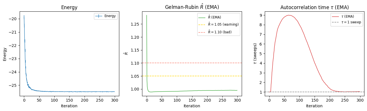
../_images/c92ce7c8c0b927a788e572a925e3f3e2ff8dbe0380b65dab30a11aa1a2597ab5.png

The Energy_ema statistics give you a live sampling health-check during optimization:

\(\hat{R} \lesssim 1.05\) — chains are well-mixed: good.
\(\hat{R} > 1.1\) — chains are not mixing: consider increasing sweep_size or n_discard_per_chain.
\(\tau_\text{corr} < 1\) sweep — consecutive samples are effectively independent: good.
\(\tau_\text{corr} > 1\) sweep — samples are correlated; consider increasing sweep_size.

Note

The EMA window averages across consecutive optimization steps, so it can mix information from slightly different wavefunctions. For a more reliable diagnosis on the final converged state, use check_mc_convergence() as described below.

Post-optimization check: `check_mc_convergence`#

After optimization has converged, you should verify that the final variational state samples well. The method check_mc_convergence() does this by:

Working on a temporary copy of the state (the original is never mutated).
Resetting the internal sweep size to 1, so every elementary MC step is an individual sample — this exposes short-range correlations.
Accumulating batches of local estimators and feeding them into an online statistics engine that tracks mean, variance, \(\hat{R}\), and the integrated autocorrelation time \(\tau_\text{corr}\) via Geyer’s initial positive sequence (IPS) estimator.
Adaptively doubling the sweep size if the autocorrelation window saturates (i.e., the chains are still strongly correlated at the maximum lag).
Stopping when the \(\tau_\text{corr}\) estimate is reliable — roughly when there are at least 50 effective samples per chain.

The function requires chains of at least ~100 steps to reliably estimate \(\hat{R}\) and \(\tau_\text{corr}\). This is perfectly fine when called post-optimization, since we are no longer constrained by the per-iteration speed budget.

Let’s run it now on the converged state:

# check_mc_convergence works on a copy of vs — it does not modify vs
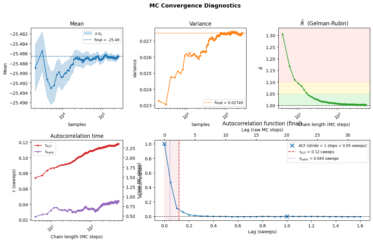
stats, hist = vs.check_mc_convergence(ha, min_chain_length=500, plot=True)

  Reached maximum chain length (500 samples/chain). Stopping.

---- MC Convergence Results ----
  Final statistics         : -25.48661 ± 0.00054 [σ²=2.7e-02, R̂=1.002]

  τ_corr (MC steps)        : 2.35

  MCState.sweep_size       : 20
  τ_corr (MC sweeps)       : 0.118  ✅  (< 1 sweep — good)

  Minimum sweep_size       : ~4.7  (= 2 × τ_corr in MC steps)

  In NQS, keep sweep_size ≥ 2τ (MC steps) so that consecutive samples
  are effectively independent and all samples carry useful information.
--------------------------------

/Users/filippo.vicentini/Nextcloud/Codes/Python/netket/netket/_src/vqs/plot_mc_convergence.py:279: UserWarning: This figure includes Axes that are not compatible with tight_layout, so results might be incorrect.
  fig.tight_layout()

../_images/b80dd337973bde6698795c3ebe3136dad3bf3a23ac8e40edc2151ce409cabef4.png

Notice that everything computed and reported here is relative to the operator we provided to the function, in this case to the energy. Different operators might expose different MC convergence issues! The figure produced by plot=True has five panels:

Mean: Should stabilise as more samples are accumulated.
Variance: Should stabilise similarly.
\(\hat{R}\): (Gelman-Rubin) | Should approach 1. Values \(< 1.05\) (green band) are good; \(> 1.1\) (red) indicates poor mixing. You should see that for short chains (\(<20\) in this example) the Gelman-Rubin R estimator is overestimated and unreliable. That motivates the online estimation discussed above.
\(\tau_\text{corr}\): Correlation time in sweep units. Values \(< 1\) mean consecutive samples are effectively independent — good. We report two esitmates of the autocorrelation time, one due to Gellman and Rubin based on the variance among chains, which is at most 1/2 of the real autocorrelation time computed by convolving the data across small windows.
Autocorrelation function: Should decay to zero within the lag window. A shaded region highlights \(\tau_\text{ACF}\).

We report the autocorrelation time and function both in units of the sweeps, as well as in units of the raw MC steps. Consider that a sweep is sampler.sweep_size MC steps. In general you want your sweep size to be larger than 2x the autocorrelation time AT THE LEAST otherwise you are effectivelly wasting compute time.

This function also tells you:

The correlation time in raw MC steps.
Whether your current sweep_size is large enough.
The recommended minimum sweep_size (= \(2\tau_\text{MC}\) raw steps).

A healthy output looks like:

  τ_corr (MC sweeps)       : 0.3  ✅  (< 1 sweep — good)

whereas a problematic one reads:

  τ_corr (MC sweeps)       : 2.1  ❌  (≥ 1 sweep — consider increasing sweep_size)

Thermalising chains before measuring: `thermalise`#

Sometimes, for example after loading a checkpoint or initialising with a biased configuration, the Markov chains start far from the typical configurations of the final wavefunction. In those cases check_mc_convergence() will report a large \(\hat{R}\), telling you the chains are not mixed yet.

thermalise() solves this by running the sampler and monitoring \(\hat{R}\) via a sliding EMA window, stopping once \(\hat{R} <\) rhat_tol has been sustained for patience consecutive iterations. Unlike check_mc_convergence(), calling this method thermalises the state in-place, ready for measurements.

Note

thermalise uses the current sweep_size. If thermalisation is slow, consider increasing sweep_size or switching to a better transition rule such as HamiltonianRule.

A typical use case is loading a checkpoint and thermalising before measuring:

# Chains start from random positions — thermalise before measuring
vs = nk.vqs.MCState(sa, ma, n_samples=1024, variables=loaded_variables)
stats, hist = vs.thermalise(ha, max_chain_length=2000, verbose=True)
e = vs.expect(ha)

The method returns a (stats, hist) tuple just like check_mc_convergence. You can plot \(\hat{R}\) over time from hist["R_hat"].values to verify convergence.

# Bias chains to all-up to simulate a bad start
import numpy as np
all_up = np.ones((vs.sampler.n_chains, hi.size), dtype=np.int8)
vs.sampler_state = vs.sampler_state.replace(σ=all_up)

# Thermalise: mutates vs.sampler_state in-place
stats_th, hist_th = vs.thermalise(ha, max_chain_length=2000, verbose=True)

print(f"Final R_hat after thermalisation: {stats_th.R_hat:.4f}")

High-precision estimation: `expect_to_precision`#

Once you are satisfied that the chains are mixing well, you may want to compute an observable to a specific statistical precision. Simply running vs.expect(op) with a fixed number of samples gives you whatever error the current n_samples yields. With expect_to_precision() you instead specify the desired error and let NetKet sample until that precision is reached.

The method accepts:

atol — desired absolute standard error on the mean.
rtol — desired relative standard error (i.e. error / |mean|).
Both can be given simultaneously; sampling continues until both are satisfied.

It works by iteratively drawing new batches of samples and updating an online statistics accumulator, showing a progress bar as it goes.

Let us compute the staggered magnetisation \(M_z = \frac{1}{L}\sum_i (-1)^i \hat{\sigma}^z_i\) to a 1% relative precision:

# Staggered magnetisation
mag = sum((-1)**i * nk.operator.spin.sigmaz(hi, i) for i in range(L)) / L

# Sample until |error / mean| <= 1 %
online_stats = vs.expect_to_precision(mag, rtol=0.01)

# Get the final Stats object
result = online_stats.get_stats()
print(result)

The returned OnlineStatistics accumulator can also give you \(\hat{R}\) and \(\tau_\text{corr}\) at the end of the sampling:

print(f"Mean              : {result.mean:.6f}")
print(f"Error of mean     : {result.error_of_mean:.2e}")
print(f"R-hat             : {online_stats.R_hat:.5f}")
print(f"tau_corr (ACF)    : {online_stats.tau_corr_acf:.3g} sweeps")

Summary and practical advice#

The table below summarises when to use each tool:

Situation	Tool	Notes
During optimization, chains are short (2–8 steps)	`Energy_ema` in `VMC_SR` log	Proxy diagnostics from pooled samples across iterations
After optimization, chains may be stuck / bimodal	`thermalise()`	Mutates state in-place; advances chains until \(\hat{R}\) converges
After optimization, verify final state quality	`check_mc_convergence()`	Needs long chains (~100–500 steps); works on a copy
Need a precise expectation value with known error	`expect_to_precision()`	Samples until `atol`/`rtol` is met

Regarding Rhat, the mixing indicator:

Diagnostic	Healthy	Warning	Bad
\(\hat{R}\)	\(< 1.05\)	\(1.05\)–\(1.1\)	\(> 1.1\)
\(\tau_\text{corr}\) (sweeps)	\(< 1\)	—	\(\geq 1\)

If diagnostics are bad#

If \(\hat{R}\) is large, you need to:

Thermalise your chains using thermalise(), which advances the chains until \(\hat{R}\) converges
Switch to a better transition rule — e.g., HamiltonianRule explores the Hilbert space more effectively than LocalRule for some problems.
Check your model — very high-variance models can make the energy landscape rugged and slow down mixing.

If \(\tau_\text{corr}\) exceeds one sweep, try one or more of the following:

Increase sweep_size — the recommended minimum is \(2\tau_\text{MC}\) raw steps, as reported by check_mc_convergence.
Increase n_discard_per_chain — discard more steps at the start of each chain to reduce the effect of the initial state.

Checking Monte Carlo convergence

Contents

Checking Monte Carlo convergence#

The chain-length problem in VMC#

The Energy_ema diagnostic during optimization#

Post-optimization check: check_mc_convergence#

Thermalising chains before measuring: thermalise#

High-precision estimation: expect_to_precision#