Infidelity Minimization with Stochastic Reconfiguration in NetKet

Authors: Luca Gravina and Alessandro Sinibaldi, August 2025

This tutorial demonstrates how to minimize the infidelity between a variational quantum state and a target state using NetKet.

• Fidelity between two states \(|\psi\rangle\) and \(|\phi\rangle\) is \(F = |\langle \psi | \phi \rangle|^2/\langle \psi | \psi \rangle \langle \phi | \phi \rangle\). The infidelity is \(1 - F\) and is minimized when the two states coincide up to a global phase.

• We will:

  1. Define a lattice, Hilbert space, variational model \(|\psi(\theta)\rangle\), and Hamiltonian \(H\).

  2. Construct a target state \(| \psi_\mathrm{target} \rangle\) from exact diagonalization (ground state of \(H\)).

  3. Optimize the variational parameters by minimizing infidelity \(1 - |\langle \psi(\theta) | \psi_\mathrm{target} \rangle|^2/ \langle \psi(\theta) | \psi(\theta) \rangle \langle \psi_\mathrm{target} | \psi_\mathrm{target} \rangle\) using the driver nk.driver.Infidelity_SR implementing infidelity minimization with Stochastic Reconfiguration (see Sinibaldi et al. and Gravina et al. for details). We consider also the case where we learn \(O | \psi_\mathrm{target} \rangle\) for a given local operator \(O\).

  4. Monitor convergence via the infidelity curve and validate energies against exact results.

Setup and imports

We import the core NetKet library and experimental drivers, JAX/NumPy for array operations, and Matplotlib for plots.

import netket as nk

print("Notebook run with NetKet version:", nk.__version__)

import jax.numpy as jnp
import numpy as np

import matplotlib.pyplot as plt

System, model definition and target state

We set up the physical problem:

• \(L\times L\) square lattice of spins-\(\tfrac{1}{2}\).

• Variational ansatz: Restricted Boltzmann Machine with real parameters.

• Transverse-field Ising Hamiltonian \(H\).

L = 4
g = nk.graph.Square(
    length=L,
)
hi = nk.hilbert.Spin(0.5, N=g.n_nodes)

ma = nk.models.RBM(alpha=3, param_dtype=jnp.float64)
n_samples = 2**13

H = nk.operator.Ising(hilbert=hi, graph=g, J=-1.0, h=3.04438)

Target and variational states

• Compute the exact ground state \(|\psi_\mathrm{target}\rangle\) via Lanczos ED.

• Build two MCState objects:

  • vs_target: LogStateVector initialized with exact amplitudes to represent \(|\psi_\mathrm{target}\rangle\).

  • vs: RBM variational state \(|\psi(\theta)\rangle\) to be optimized.

sa = nk.sampler.MetropolisLocal(hilbert=hi, n_chains_per_rank=16)
ma = nk.models.RBM(alpha=3, param_dtype=jnp.float64)

e_gs, v_gs = nk.exact.lanczos_ed(H, compute_eigenvectors=True)

vs_target = nk.vqs.MCState(
    sampler=sa,
    model=nk.models.LogStateVector(hi, param_dtype=jnp.float64),
    n_samples=n_samples,
    variables={"params": {"logstate": jnp.log(v_gs.astype(jnp.complex128)).squeeze()}},
)

vs = nk.vqs.MCState(
    sampler=sa,
    model=ma,
    n_samples=n_samples,
)

Infidelity minimization (no operator)

We now minimize the infidelity \(1 - |\langle \psi(\theta) | \psi_\mathrm{target} \rangle|^2 / \langle \psi(\theta) | \psi(\theta) \rangle \langle \psi_\mathrm{target} | \psi_\mathrm{target} \rangle\) using Stochastic Reconfiguration (SR):

• The SR metric preconditions parameter updates to approximate the natural gradient on the variational manifold.

• The regularization (diagonal shift) \(\lambda_\mathrm{SR}\) stabilizes the metric inversion.

We run the driver for a fixed number of iterations and record the infidelity statistics.

optimizer = nk.optimizer.Sgd(learning_rate=5e-2)
diag_shift = 1e-4

logger = nk.logging.RuntimeLog()
driver = nk.driver.Infidelity_SR(
    target_state=vs_target,
    optimizer=optimizer,
    diag_shift=diag_shift,
    variational_state=vs,
    operator=None,
)
driver.run(n_iter=100, out=logger)

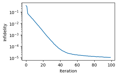
Monitoring convergence

We plot the infidelity versus iteration. A fast decay toward small values indicates \(|\psi(\theta)\rangle\) matches \(|\psi_\mathrm{target}\rangle\) up to a global phase.

infidelity = logger["Infidelity"]["Mean"]
error = logger["Infidelity"]["Sigma"]

fig, ax = plt.subplots(1, 1, figsize=(4, 2.5))
ax.plot(range(len(infidelity)), infidelity, "-")
ax.fill_between(
    range(len(infidelity)), infidelity - error, infidelity + error, alpha=0.3
)
ax.set_yscale("log")
ax.set_xlabel("Iteration")
ax.set_ylabel("Infidelity");

Energy validation (ground state)

As a sanity check, we compute the energy of the learned variational state \(E_\mathrm{VMC} = \langle \psi(\theta) | H | \psi(\theta) \rangle\) and compare it to the exact ground-state energy \(E_0\) from ED. Agreement within tolerance confirms successful state learning.

psi = vs.to_array()
energy = psi.T @ H.to_sparse() @ psi

np.testing.assert_allclose(energy, e_gs, rtol=1e-5)

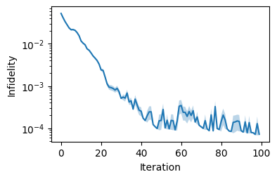
Infidelity minimization with an operator

Sometimes we wish to match the state proportional to \(O\,|\psi_\mathrm{target}\rangle\) for a physical operator \(O\) (e.g., a transition operator). We define

• \(O = \sum_i \sigma_i^+\) Then we repeat the optimization, now minimizing the infidelity to the normalized vector \(\dfrac{O\,|\psi_\mathrm{target}\rangle}{\|O\,|\psi_\mathrm{target}\rangle\|}\).

operator = sum([nk.operator.spin.sigmap(hi, i) for i in g.nodes()])

optimizer = nk.optimizer.Sgd(learning_rate=5e-2)
diag_shift = 1e-6

logger = nk.logging.RuntimeLog()
driver = nk.driver.Infidelity_SR(
    target_state=vs_target,
    optimizer=optimizer,
    diag_shift=diag_shift,
    variational_state=vs,
    operator=operator,
)
driver.run(n_iter=100, out=logger)

infidelity = logger["Infidelity"]["Mean"]
error = logger["Infidelity"]["Sigma"]

fig, ax = plt.subplots(1, 1, figsize=(4, 2.5))
ax.plot(range(len(infidelity)), infidelity, "-")
ax.fill_between(
    range(len(infidelity)), infidelity - error, infidelity + error, alpha=0.3
)
ax.set_yscale("log")
ax.set_xlabel("Iteration")
ax.set_ylabel("Infidelity");

Energy validation (operator-transformed target)

We construct the exact reference state \(|\psi_\mathrm{ref}\rangle \propto O\,|\psi_\mathrm{target}\rangle\) and compare its energy \(E_\mathrm{ref} = \langle \psi_\mathrm{ref} | H | \psi_\mathrm{ref} \rangle\) to that of the trained variational state \(E_\mathrm{VMC} = \langle \psi(\theta) | H | \psi(\theta) \rangle\).

psi_target = operator.to_sparse() @ vs_target.to_array()
psi_target = psi_target / np.linalg.norm(psi_target)

energy_exact = psi_target.T @ H.to_sparse() @ psi_target

psi = vs.to_array()
energy_variational = psi.T @ H.to_sparse() @ psi

np.testing.assert_allclose(energy_variational, energy_exact, rtol=1e-3)